Multilayer perceptron

This notebook illustrates the creation and the training of a regular multilayer perceptron.

import os
import sys

sys.path.append(os.path.join(os.path.abspath(""), ".."))

import numpy as np
from IPython.display import Markdown as md

from torch import nn, optim

from nnbma.networks import FullyConnected
from nnbma.dataset import RegressionDataset
from nnbma.learning import learning_procedure, LearningParameters

from functions import Fexample as F

Analytical function

In the following cell, we load and instantiate a vectorial function \(f\) implemented as a PyTorch Module. For more details on the implementation, see functions.py. You can implement your own by following the model.

The function is the following:

f = F()
md(F.latex())

\[\begin{split}\left(\begin{array}{c} t_1\\ t_2 \end{array}\right) \longmapsto \left(\begin{array}{c} t_1+2t_2\\ t_1^2\\ t_1t_2^2 \end{array}\right)\end{split}\]

Definition of the architecture

The multilayer perceptron is historically the most common architecture. Every layer is fully connected to the previous one (that why is it often called “fully connected neural network”).

Below, an example from the related paper for 2 inputs, 10 outputs and 2 hidden layers of respective sizes 4 and 8:

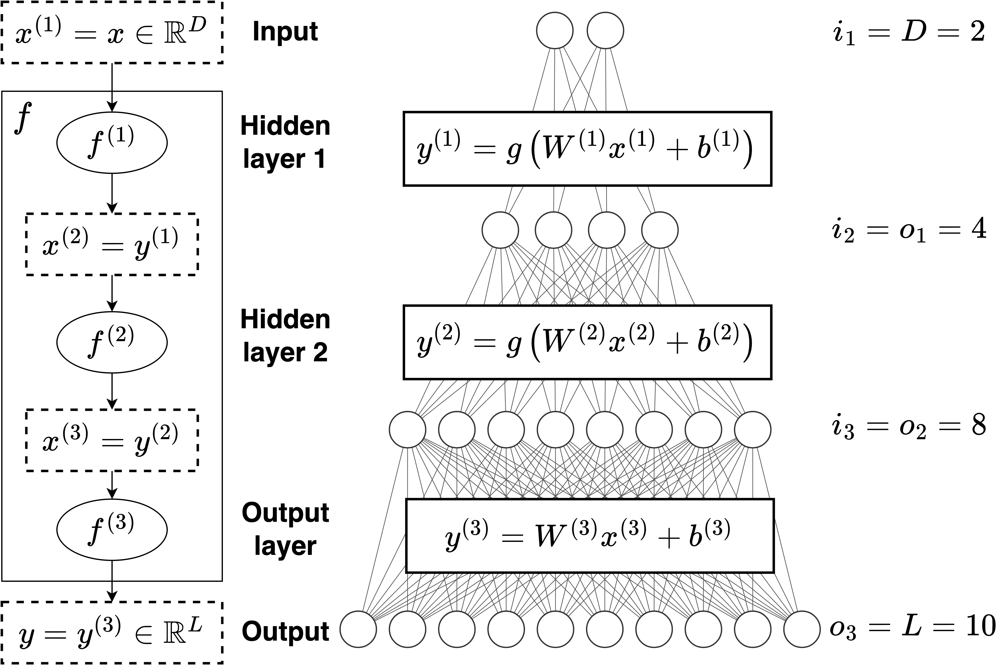
The transition between two layer is composed of a matrix product and an activation function such as \(\mathrm{ReLU}\), \(\mathrm{tanh}\) or any of their numerous variants.

The parameters that you can tuned in order to improve your model are the following:

• the layers sizes (number of layer and number of neurons of each of them)

• the activation function (for simplicity sake, in this implementation the same function is used for every layers)

• the use of a batch normalization or not

You can also change the loss function that you use (see the section “Training procedure”).

With a FullyConnected network, as well than for any network that inherits from NeuralNetwork, you can specify the input and output features names, the device (cpu or gpu, if available) that you want to use.

Lastly, you can also specifiy whether you want the last layer to be restrictable (see the restrictable-layer.ipynb notebook in this topic).

layers_sizes = [f.n_inputs, 50, 50, f.n_outputs]  # Can be modified
activation = nn.ELU()

net = FullyConnected(layers_sizes, activation)

print(f"Number of hidden layers: {len(layers_sizes)-1}")
print(f"Layers sizes: {layers_sizes}")
print(
    f"Number of trainable weights: {net.count_parameters():,} ({net.count_bytes(display=True)})"
)

Number of hidden layers: 3
Layers sizes: [2, 50, 50, 3]
Number of trainable weights: 2,853 (11.41 kB)

Dataset

n_samples = 10_000
test_frac = 0.20

np.random.seed(0)
X = np.random.normal(0, 1, size=(n_samples, F.n_inputs)).astype("float32")
Y = f(X)

X_train, X_test = X[round(test_frac * n_samples) :], X[: round(test_frac * n_samples)]
Y_train, Y_test = Y[round(test_frac * n_samples) :], Y[: round(test_frac * n_samples)]

train_dataset = RegressionDataset(X_train, Y_train)
test_dataset = RegressionDataset(X_test, Y_test)

print(f"Number of training entries: {X_train.shape[0]:,}")
print(f"Number of testing entries: {X_test.shape[0]:,}")

Number of training entries: 8,000
Number of testing entries: 2,000

Training procedure

# Epochs
epochs = 100

# Batch size
batch_size = 100

# Loss function
loss = nn.MSELoss()

# Optimizer
learning_rate = 1e-3
optimizer = optim.Adam(net.parameters(), learning_rate)

learning_params = LearningParameters(loss, epochs, batch_size, optimizer)

results = learning_procedure(
    net,
    (train_dataset, test_dataset),
    learning_params,
    val_frac=test_frac,
)

Results

def metric(y_hat: np.ndarray, y: np.ndarray):
    return np.mean((y_hat - y) ** 2)

print(f"Loss over training set: {metric(net(X_train), Y_train):.2e}")
print(f"Loss over testing set: {metric(net(X_test), Y_test):.2e}")

Loss over training set: 8.36e-04
Loss over testing set: 2.94e-03