Neural networks auto-differentiation using PyTorch 2.0
Before running this notebook, you must run training.ipynb in order to generate the function and the network that will be loaded and derived in this notebook. Note that the tools that will be use are only available for torch >= 2.0.
[1]:
import os
import sys

sys.path.append(os.path.join(os.path.abspath(""), ".."))

import shutil

import numpy as np
import matplotlib.pyplot as plt
from IPython.display import Markdown as md

import torch
from torch.func import jacrev, hessian, vmap

import numpy as np

from nnbma.networks import NeuralNetwork

from functions import Fexample as F

plt.rc("text", usetex=shutil.which("latex") is not None)
dpi = 150
Introduction to differentiation with PyTorch
We will use the following modules: * jacrev: compute the jacobian using reverse-mode autodiff * jacfwd: compute the jacobian using forward-mode autodiff * hessian: compute the jacobian using both reverse and forward-mode autodiff * vmap: vectorizing function used to compute the derivatives of batched inputs
The computation of high order derivative can be done by composing several times jacrev and/or jacfwd. Note that hessian is just a convenience module defined as hessian(f) = jacfwd(jacrev(f)), but that the hessian computation can be done through other compositions.
Import of the analytical function
In the following cell, we will import the vectorial function \(f\). Please refer to training.ipynb for more details on it. If you’ve created your own function, please be sure to import this one.
The function is the following:
[2]:
md(F.latex())
[2]:
[3]:
f = F()

ranges = [
    (-2.0, 2.0),
    (-1.0, 1.0),
]  # Range of values of all inputs of f. Can be modified but must be consistent with the imported function.

n_points = 100  # Number of points needed to plot a profile

default_values = [
    1.0,
    1.0,
]  # Default values of all inputs of f when plotting a profile. Can be modified but must be consistent with the imported function.
Loading of the trained network
[4]:
path = os.path.join(os.path.splitext(os.path.abspath(""))[0], "out-training")

net = NeuralNetwork.load("network", path)
net.double().eval()
print(net)
FullyConnected:
        layers_sizes: [2, 100, 100, 3]
        activation: GELU(approximate='none')
        batch_norm: False
        inputs_names: None
        outputs_names: None
        inputs_transformer: None
        outputs_transformer: None
        device: cpu
        last_restrictable: True
Differentiation of the analytical function
In this part, we will compute the first and second order derivatives of the analytical function defined in training.ipynb. As the number of possible plots explodes when we differentiate a vectorial function several times, we will chose to represent only the evolution of a single output versus only one or two variables.
[5]:
# Index of free input when plotting profiles, the others being restricted to their default value.
input_to_plot = 1  # Must be between 1 and f.n_inputs

# Index of free inputs when drawing bivariate plots, the others being restricted to their default value.
inputs_to_plot = (1, 2)  # Must be between 1 and f.n_inputs

# Index of the output to plot.
output_to_plot = 3  # Must be between 1 and f.n_outputs
[6]:
jacobian_f = vmap(jacrev(f))
hessian_f = vmap(hessian(f))
Profiles of first and second order derivatives
[7]:
x = np.array(default_values) * np.ones((n_points, f.n_inputs), dtype="float")
x[:, input_to_plot - 1] = np.linspace(*ranges[input_to_plot - 1], n_points)
print("x.shape:", x.shape)

dy = jacobian_f(torch.from_numpy(x)).detach().numpy()
print("dy.shape:", dy.shape)

ddy = hessian_f(torch.from_numpy(x)).detach().numpy()
print("ddy.shape:", ddy.shape)
x.shape: (100, 2)
dy.shape: (100, 3, 2)
ddy.shape: (100, 3, 2, 2)
[8]:
plt.figure(figsize=(0.7 * f.n_inputs * 6.4, 0.6 * 4.8), dpi=dpi)

for i in range(f.n_inputs):

    plt.subplot(1, f.n_inputs, i + 1)

    plt.plot(x[:, input_to_plot - 1], dy[:, output_to_plot - 1, i])

    plt.xlabel(f"$x_{input_to_plot}$")
    plt.ylabel(f"$\\partial f_{output_to_plot} / \\partial x_{i+1}$")
    plt.title(
        f"$\\partial f_{output_to_plot} / \\partial x_{i+1}$ vs $x_{input_to_plot}$"
    )

plt.tight_layout()

plt.show()
[9]:
plt.figure(figsize=(0.7 * f.n_inputs * 6.4, 0.6 * f.n_inputs * 4.8), dpi=dpi)

for i1 in range(f.n_inputs):

    for i2 in range(f.n_inputs):

        plt.subplot(f.n_inputs, f.n_inputs, i1 * f.n_inputs + i2 + 1)

        plt.plot(x[:, input_to_plot - 1], ddy[:, output_to_plot - 1, i1, i2])

        plt.xlabel(f"$x_{input_to_plot}$")
        plt.ylabel(
            f"$\\partial^2 f_{output_to_plot} / \\partial x_{i1+1} \\partial x_{i2+1}$"
        )
        plt.title(
            f"$\\partial^2 f_{output_to_plot} / \\partial x_{i1+1} \\partial x_{i2+1}$ vs $x_{input_to_plot}$"
        )

plt.tight_layout()

plt.show()
Bivariate plots of first and second order derivatives
[10]:
X = np.dstack(
    np.meshgrid(
        *[
            np.linspace(*ranges[i], n_points)
            if i + 1 in inputs_to_plot
            else default_values[i] * np.ones(n_points)
            for i in range(f.n_inputs)
        ]
    )
)
print("X.shape:", X.shape)

dY = (
    jacobian_f(torch.from_numpy(X.reshape(n_points**2, f.n_inputs)))
    .detach()
    .numpy()
    .reshape(n_points, n_points, f.n_outputs, f.n_inputs)
)
print("dY.shape:", dY.shape)

ddY = (
    hessian_f(torch.from_numpy(X.reshape(n_points**2, f.n_inputs)))
    .detach()
    .numpy()
    .reshape(n_points, n_points, f.n_outputs, f.n_inputs, f.n_inputs)
)
print("ddY.shape:", ddY.shape)
X.shape: (100, 100, 2)
dY.shape: (100, 100, 3, 2)
ddY.shape: (100, 100, 3, 2, 2)
[11]:
plt.figure(figsize=(0.7 * 6.4 * f.n_inputs, 0.7 * 4.8), dpi=dpi)

for i in range(f.n_inputs):
    plt.subplot(1, f.n_inputs, i + 1)
    plt.imshow(
        dY[:, :, output_to_plot - 1, i],
        cmap="jet",
        aspect="auto",
        extent=[
            ranges[inputs_to_plot[0] - 1][0],
            ranges[inputs_to_plot[0] - 1][1],
            ranges[inputs_to_plot[1] - 1][0],
            ranges[inputs_to_plot[1] - 1][1],
        ],
    )
    plt.colorbar()

    plt.xlabel(f"$x_{inputs_to_plot[0]}$")
    plt.ylabel(f"$x_{inputs_to_plot[1]}$")
    plt.title(
        f"$\\partial f_{output_to_plot} / \\partial x_{i+1}$ vs $x_{inputs_to_plot[0]}$ and $x_{inputs_to_plot[1]}$"
    )

plt.tight_layout()

plt.show()
[12]:
plt.figure(figsize=(0.7 * 6.4 * f.n_inputs, 0.7 * f.n_inputs * 4.8), dpi=dpi)

for i1 in range(f.n_inputs):

    for i2 in range(f.n_inputs):

        plt.subplot(f.n_inputs, f.n_inputs, i1 * f.n_inputs + i2 + 1)
        plt.imshow(
            ddY[:, :, output_to_plot - 1, i1, i2],
            cmap="jet",
            aspect="auto",
            extent=[
                ranges[inputs_to_plot[0] - 1][0],
                ranges[inputs_to_plot[0] - 1][1],
                ranges[inputs_to_plot[1] - 1][0],
                ranges[inputs_to_plot[1] - 1][1],
            ],
        )
        plt.colorbar()

        plt.xlabel(f"$x_{inputs_to_plot[0]}$")
        plt.ylabel(f"$x_{inputs_to_plot[1]}$")
        plt.title(
            f"$\\partial^2 f_{output_to_plot} / \\partial x_{i1+1} \\partial x_{i2+1}$ vs $x_{inputs_to_plot[0]}$ and $x_{inputs_to_plot[1]}$"
        )

plt.tight_layout()

plt.show()
Differentiation of the neural network
We will now compute the first and second order derivatives of a neural network that has been trained to approximate the previous function.
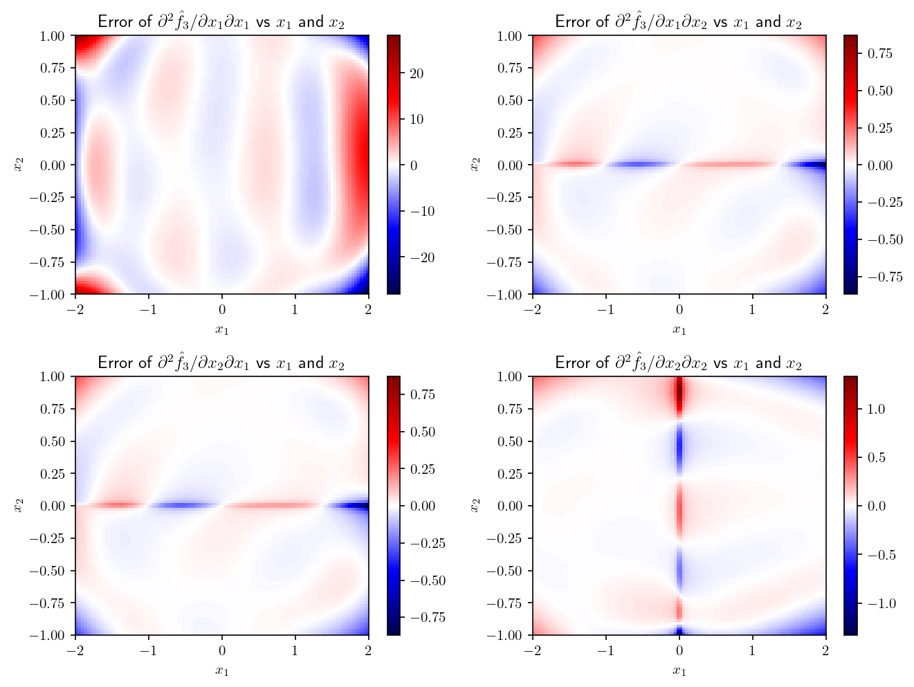
NB: Bear in mind that the error in estimating the partial derivatives depends on the model being trained. Indeed, if the model is too regularized, or on the contrary overfit the data, then the error may be significant. It should also be noted that, in general, this error increases with the order of derivation. Lastly, since learning error generally tends to be higher in regions with limited data and at the edges of the domain, the same is expected for derivative calculations.
[13]:
jacobian_net = vmap(jacrev(net.forward))
hessian_net = vmap(hessian(net.forward))
Profiles of first and second order derivatives
[14]:
x = np.array(default_values) * np.ones((n_points, f.n_inputs), dtype="float")
x[:, input_to_plot - 1] = np.linspace(*ranges[input_to_plot - 1], n_points)
print("x.shape:", x.shape)

dy_net = jacobian_net(torch.from_numpy(x)).detach().numpy()
print("dy.shape:", dy.shape)

ddy_net = hessian_net(torch.from_numpy(x)).detach().numpy()
print("ddy.shape:", ddy.shape)
x.shape: (100, 2)
dy.shape: (100, 3, 2)
ddy.shape: (100, 3, 2, 2)
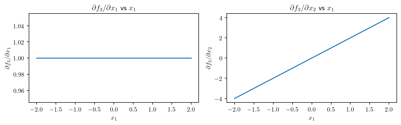
[15]:
plt.figure(figsize=(0.7 * f.n_inputs * 6.4, 0.6 * 4.8), dpi=dpi)

for i in range(f.n_inputs):

    plt.subplot(1, f.n_inputs, i + 1)

    plt.plot(x[:, input_to_plot - 1], dy_net[:, output_to_plot - 1, i])
    plt.plot(
        x[:, input_to_plot - 1],
        dy[:, output_to_plot - 1, i],
        linestyle="--",
        color="gray",
    )

    plt.xlabel(f"$x_{input_to_plot}$")
    plt.ylabel(f"$\\partial \\hat{{f}}_{output_to_plot} / \\partial x_{i+1}$")
    plt.title(
        f"$\\partial \\hat{{f}}_{output_to_plot} / \\partial x_{i+1}$ vs $x_{input_to_plot}$"
    )

plt.tight_layout()

plt.show()

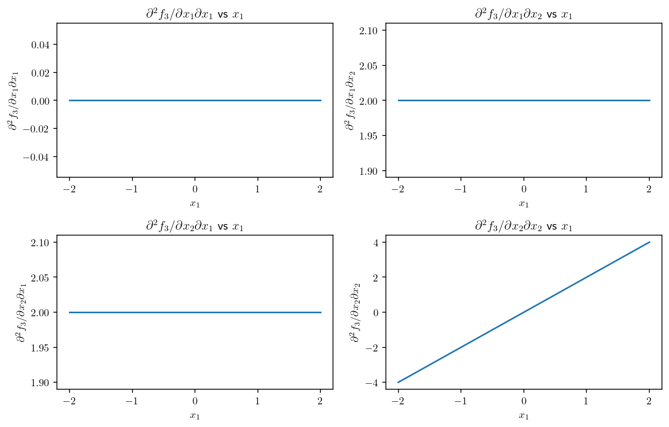
[16]:
plt.figure(figsize=(0.7 * f.n_inputs * 6.4, 0.6 * f.n_inputs * 4.8), dpi=dpi)

for i1 in range(f.n_inputs):

    for i2 in range(f.n_inputs):

        plt.subplot(f.n_inputs, f.n_inputs, i1 * f.n_inputs + i2 + 1)

        plt.plot(x[:, input_to_plot - 1], ddy_net[:, output_to_plot - 1, i1, i2])
        plt.plot(
            x[:, input_to_plot - 1],
            ddy[:, output_to_plot - 1, i1, i2],
            linestyle="--",
            color="gray",
        )

        plt.xlabel(f"$x_{input_to_plot}$")
        plt.ylabel(
            f"$\\partial^2 \\hat{{f}}_{output_to_plot} / \\partial x_{i1+1} \\partial x_{i2+1}$"
        )
        plt.title(
            f"$\\partial^2 \\hat{{f}}_{output_to_plot} / \\partial x_{i1+1} \\partial x_{i2+1}$ vs $x_{input_to_plot}$"
        )

plt.tight_layout()

plt.show()

Bivariate plots of first and second order derivatives
[17]:
X = np.dstack(
    np.meshgrid(
        *[
            np.linspace(*ranges[i], n_points)
            if i + 1 in inputs_to_plot
            else default_values[i] * np.ones(n_points)
            for i in range(f.n_inputs)
        ]
    )
)
print("X.shape:", X.shape)

dY_net = (
    jacobian_net(torch.from_numpy(X.reshape(n_points**2, f.n_inputs)))
    .detach()
    .numpy()
    .reshape(n_points, n_points, f.n_outputs, f.n_inputs)
)
print("dY.shape:", dY.shape)

ddY_net = (
    hessian_net(torch.from_numpy(X.reshape(n_points**2, f.n_inputs)))
    .detach()
    .numpy()
    .reshape(n_points, n_points, f.n_outputs, f.n_inputs, f.n_inputs)
)
print("ddY.shape:", ddY.shape)
X.shape: (100, 100, 2)
dY.shape: (100, 100, 3, 2)
ddY.shape: (100, 100, 3, 2, 2)
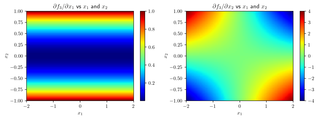
[18]:
plt.figure(figsize=(0.7 * 6.4 * f.n_inputs, 0.7 * 4.8), dpi=dpi)

for i in range(f.n_inputs):
    plt.subplot(1, f.n_inputs, i + 1)
    plt.imshow(
        dY_net[:, :, output_to_plot - 1, i],
        cmap="jet",
        aspect="auto",
        extent=[
            ranges[inputs_to_plot[0] - 1][0],
            ranges[inputs_to_plot[0] - 1][1],
            ranges[inputs_to_plot[1] - 1][0],
            ranges[inputs_to_plot[1] - 1][1],
        ],
    )
    plt.colorbar()

    plt.xlabel(f"$x_{inputs_to_plot[0]}$")
    plt.ylabel(f"$x_{inputs_to_plot[1]}$")
    plt.title(
        f"$\\partial \\hat{{f}}_{output_to_plot} / \\partial x_{i+1}$ vs $x_{inputs_to_plot[0]}$ and $x_{inputs_to_plot[1]}$"
    )

plt.tight_layout()

plt.show()

[19]:
plt.figure(figsize=(0.7 * 6.4 * f.n_inputs, 0.7 * f.n_inputs * 4.8), dpi=dpi)
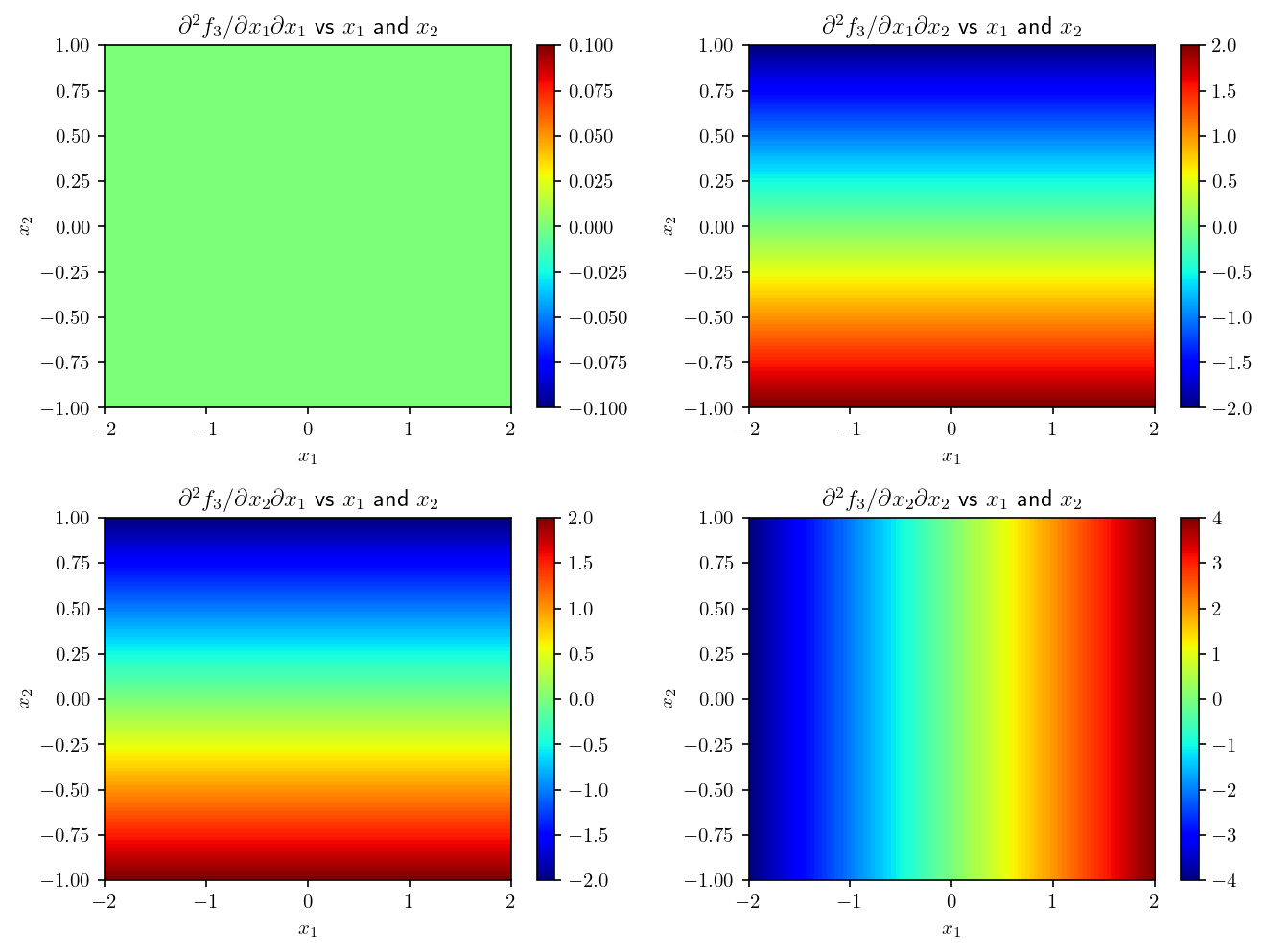
for i1 in range(f.n_inputs):
for i2 in range(f.n_inputs):
plt.subplot(f.n_inputs, f.n_inputs, i1 * f.n_inputs + i2 + 1)
plt.imshow(
ddY_net[:, :, output_to_plot - 1, i1, i2],
cmap="jet",
aspect="auto",
extent=[
ranges[inputs_to_plot[0] - 1][0],
ranges[inputs_to_plot[0] - 1][1],
ranges[inputs_to_plot[1] - 1][0],
ranges[inputs_to_plot[1] - 1][1],
],
)
plt.colorbar()
plt.xlabel(f"$x_{inputs_to_plot[0]}$")
plt.ylabel(f"$x_{inputs_to_plot[1]}$")
plt.title(
f"$\\partial^2 \\hat{{f}}_{output_to_plot} / \\partial x_{i1+1} \\partial x_{i2+1}$ vs $x_{inputs_to_plot[0]}$ and $x_{inputs_to_plot[1]}$"
)
plt.tight_layout()
plt.show()

Errors of approximated derivatives
[20]:
relative = True
eps = 1e-2
Profiles of first and second order derivatives
[21]:
error_dy = (dy_net - dy) / (np.abs(dy) + eps) if relative else dy_net - dy
print("error_dy.shape:", error_dy.shape)

error_ddy = (ddy_net - ddy) / (np.abs(ddy) + eps) if relative else ddy_net - ddy
print("error_ddy.shape:", error_ddy.shape)
error_dy.shape: (100, 3, 2)
error_ddy.shape: (100, 3, 2, 2)
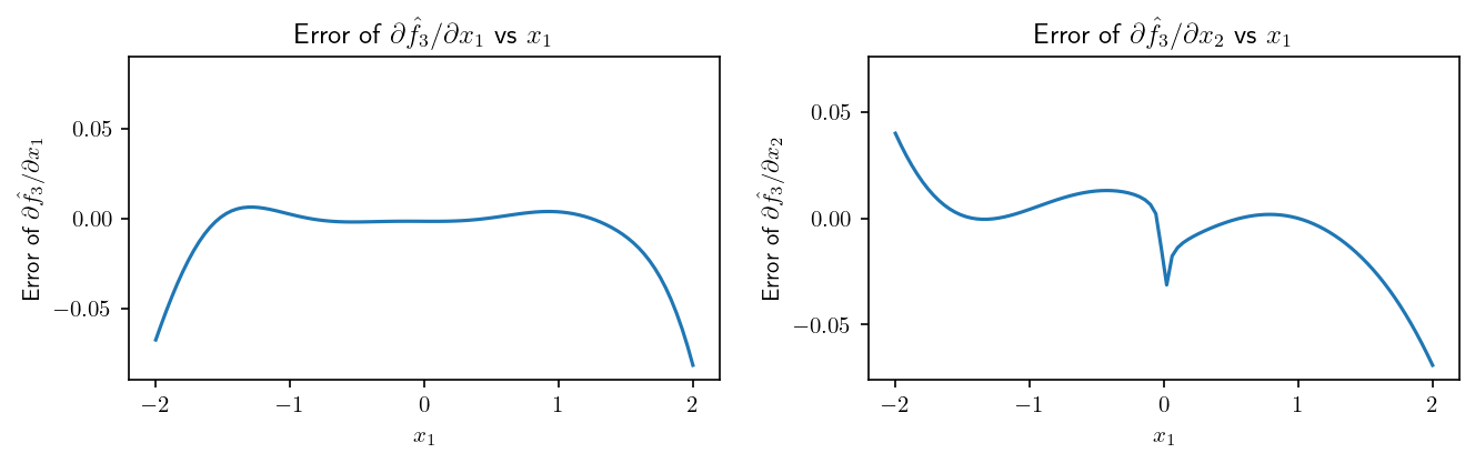
[22]:
plt.figure(figsize=(0.7 * f.n_inputs * 6.4, 0.6 * 4.8), dpi=dpi)

for i in range(f.n_inputs):

    vmax = np.abs(error_dy[:, output_to_plot - 1, i]).max()

    plt.subplot(1, f.n_inputs, i + 1)

    plt.plot(x[:, input_to_plot - 1], error_dy[:, output_to_plot - 1, i])
    plt.ylim([-1.1 * vmax, 1.1 * vmax])

    plt.xlabel(f"$x_{input_to_plot}$")
    plt.ylabel(f"Error of $\\partial \\hat{{f}}_{output_to_plot} / \\partial x_{i+1}$")
    plt.title(
        f"Error of $\\partial \\hat{{f}}_{output_to_plot} / \\partial x_{i+1}$ vs $x_{input_to_plot}$"
    )

plt.tight_layout()

plt.show()
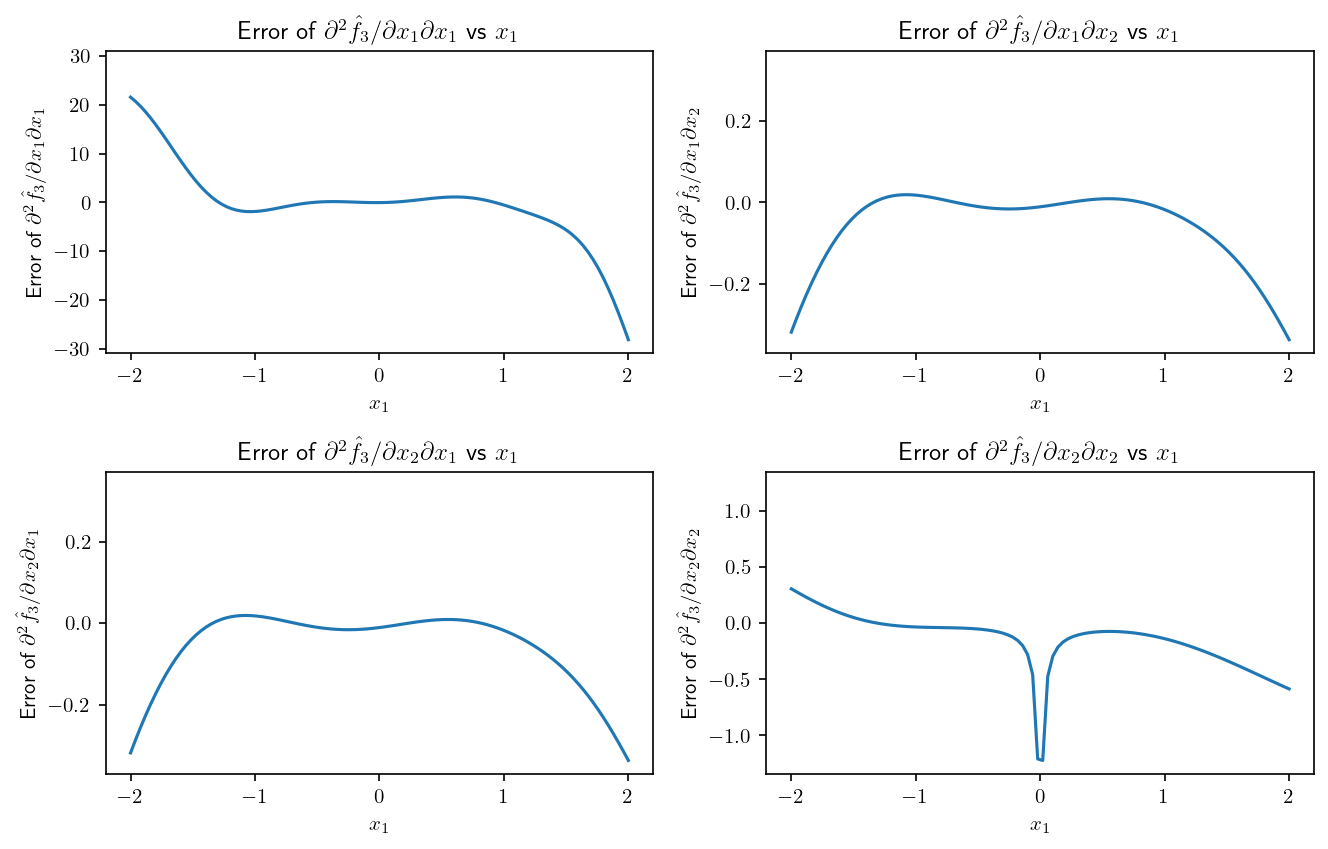
[23]:
plt.figure(figsize=(0.7 * f.n_inputs * 6.4, 0.6 * f.n_inputs * 4.8), dpi=dpi)

for i1 in range(f.n_inputs):

    for i2 in range(f.n_inputs):

        vmax = np.abs(error_ddy[:, output_to_plot - 1, i1, i2]).max()

        plt.subplot(f.n_inputs, f.n_inputs, i1 * f.n_inputs + i2 + 1)

        plt.plot(x[:, input_to_plot - 1], error_ddy[:, output_to_plot - 1, i1, i2])
        if vmax > 0:
            plt.ylim([-1.1 * vmax, 1.1 * vmax])

        plt.xlabel(f"$x_{input_to_plot}$")
        plt.ylabel(
            f"Error of $\\partial^2 \\hat{{f}}_{output_to_plot} / \\partial x_{i1+1} \\partial x_{i2+1}$"
        )
        plt.title(
            f"Error of $\\partial^2 \\hat{{f}}_{output_to_plot} / \\partial x_{i1+1} \\partial x_{i2+1}$ vs $x_{input_to_plot}$"
        )

plt.tight_layout()

plt.show()
Bivariate plots of first and second order derivatives
[24]:
Error_dY = (dY_net - dY) / (np.abs(dY) + eps) if relative else dY_net - dY
print("Error_dY.shape:", dY.shape)

Error_ddY = (ddY_net - ddY) / (np.abs(ddY) + eps) if relative else ddY_net - ddY
print("Error_ddY.shape:", ddY.shape)
Error_dY.shape: (100, 100, 3, 2)
Error_ddY.shape: (100, 100, 3, 2, 2)
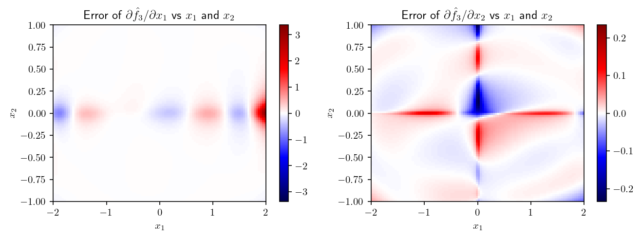
[25]:
plt.figure(figsize=(0.7 * 6.4 * f.n_inputs, 0.7 * 4.8), dpi=dpi)

for i in range(f.n_inputs):

    vmax = np.abs(Error_dY[:, :, output_to_plot - 1, i]).max()

    plt.subplot(1, f.n_inputs, i + 1)
    plt.imshow(
        Error_dY[:, :, output_to_plot - 1, i],
        cmap="seismic",
        aspect="auto",
        extent=[
            ranges[inputs_to_plot[0] - 1][0],
            ranges[inputs_to_plot[0] - 1][1],
            ranges[inputs_to_plot[1] - 1][0],
            ranges[inputs_to_plot[1] - 1][1],
        ],
        vmin=-vmax,
        vmax=vmax,
    )
    plt.colorbar()

    plt.xlabel(f"$x_{inputs_to_plot[0]}$")
    plt.ylabel(f"$x_{inputs_to_plot[1]}$")
    plt.title(
        f"Error of $\\partial \\hat{{f}}_{output_to_plot} / \\partial x_{i+1}$ vs $x_{inputs_to_plot[0]}$ and $x_{inputs_to_plot[1]}$"
    )

plt.tight_layout()

plt.show()
[26]:
plt.figure(figsize=(0.7 * 6.4 * f.n_inputs, 0.7 * f.n_inputs * 4.8), dpi=dpi)

for i1 in range(f.n_inputs):

    for i2 in range(f.n_inputs):

        vmax = np.abs(Error_ddY[:, :, output_to_plot - 1, i1, i2]).max()

        plt.subplot(f.n_inputs, f.n_inputs, i1 * f.n_inputs + i2 + 1)
        plt.imshow(
            Error_ddY[:, :, output_to_plot - 1, i1, i2],
            cmap="seismic",
            aspect="auto",
            extent=[
                ranges[inputs_to_plot[0] - 1][0],
                ranges[inputs_to_plot[0] - 1][1],
                ranges[inputs_to_plot[1] - 1][0],
                ranges[inputs_to_plot[1] - 1][1],
            ],
            vmin=-vmax,
            vmax=vmax,
        )
        plt.colorbar()

        plt.xlabel(f"$x_{inputs_to_plot[0]}$")
        plt.ylabel(f"$x_{inputs_to_plot[1]}$")
        plt.title(
            f"Error of $\\partial^2 \\hat{{f}}_{output_to_plot} / \\partial x_{i1+1} \\partial x_{i2+1}$ vs $x_{inputs_to_plot[0]}$ and $x_{inputs_to_plot[1]}$"
        )

plt.tight_layout()

plt.show()